Optimisation of Bus Timetables:
An Adaptive Large Neighbourhood Search-based Matheuristic with a Novel Operator Weight
Mr. Robin Gaborit
Technical University of Denmark
Dr. Yu Jiang
Lancaster University
Motivation
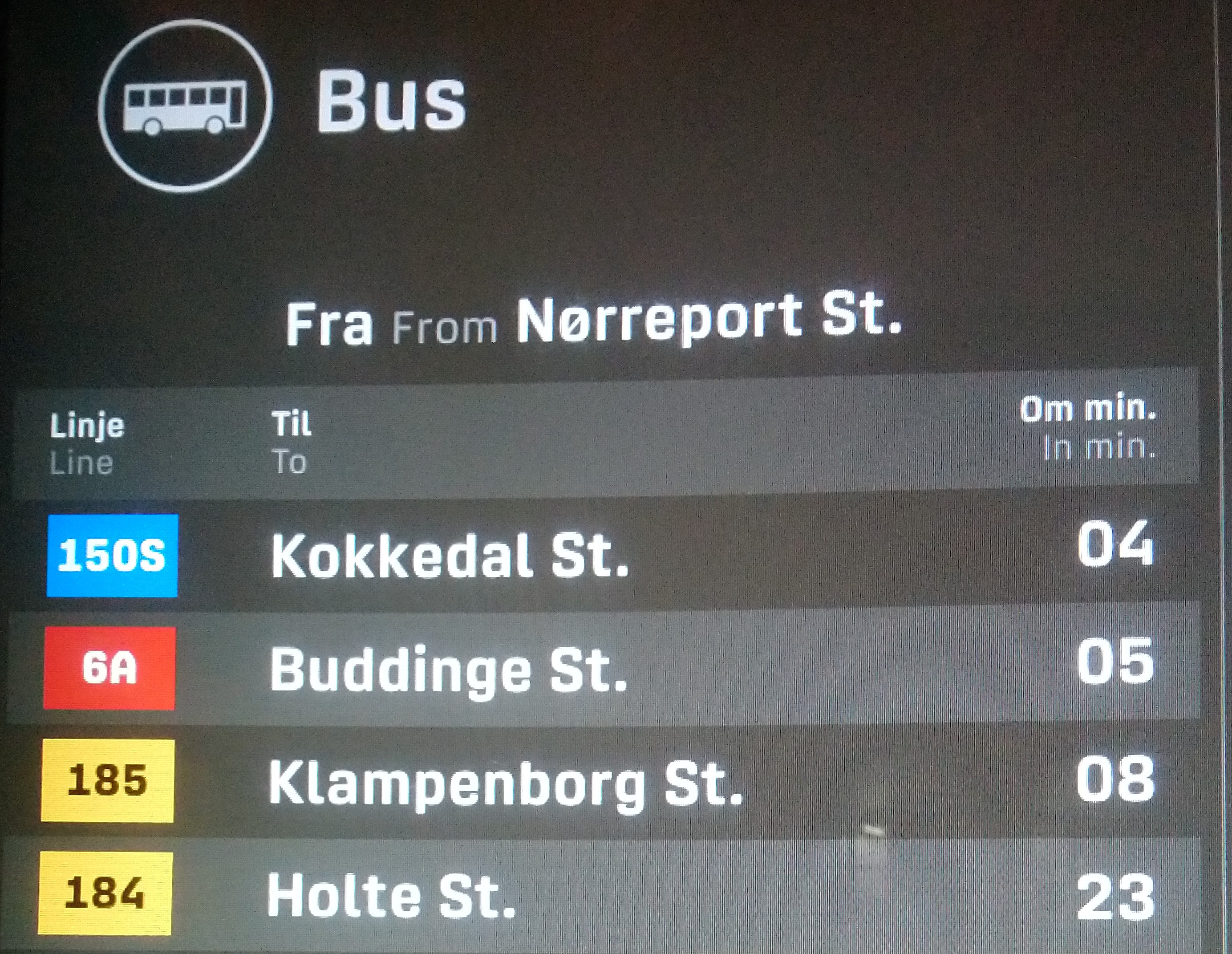
The Bus Timetabling Problem
- Problem: Transfer waiting times significantly impact passenger experience
- Decision: Set departure/arrival times of buses from/at stops
- Objective: Minimize (weighted) passenger travel times
- Challenge: Model is too complex for exact solutions → Need for metaheuristics
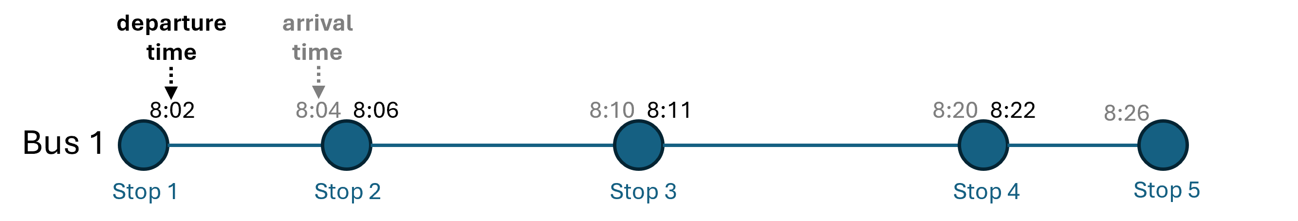
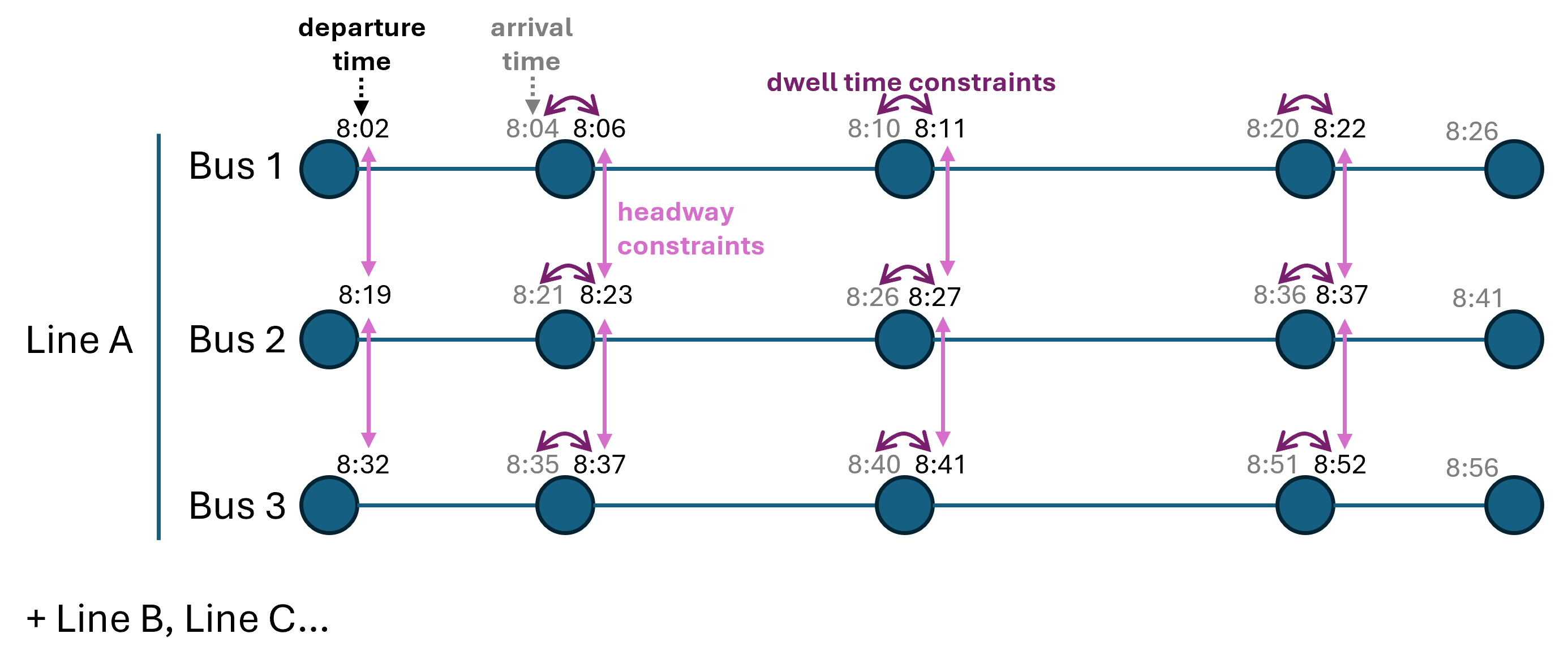
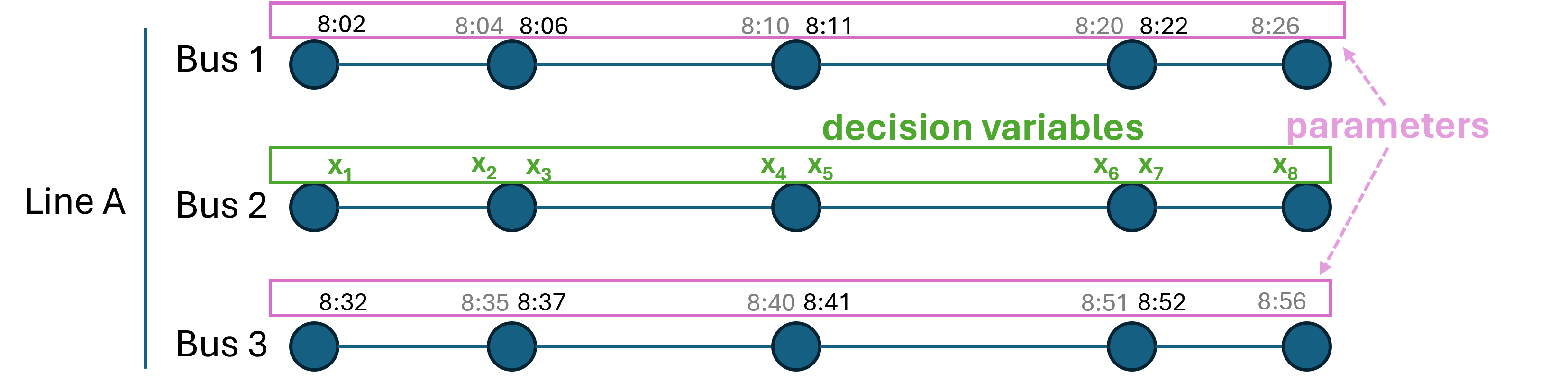
Decision Variables
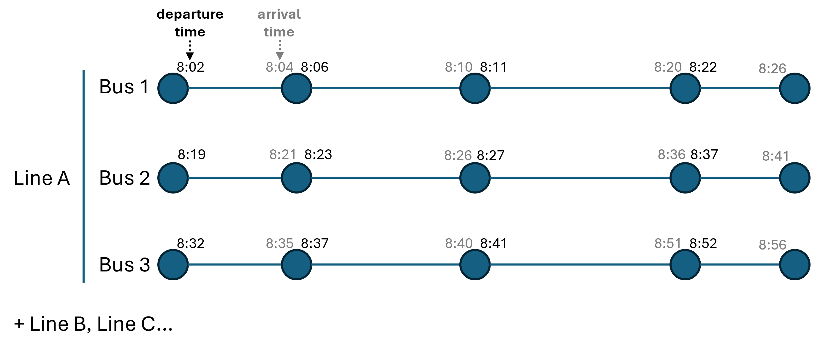
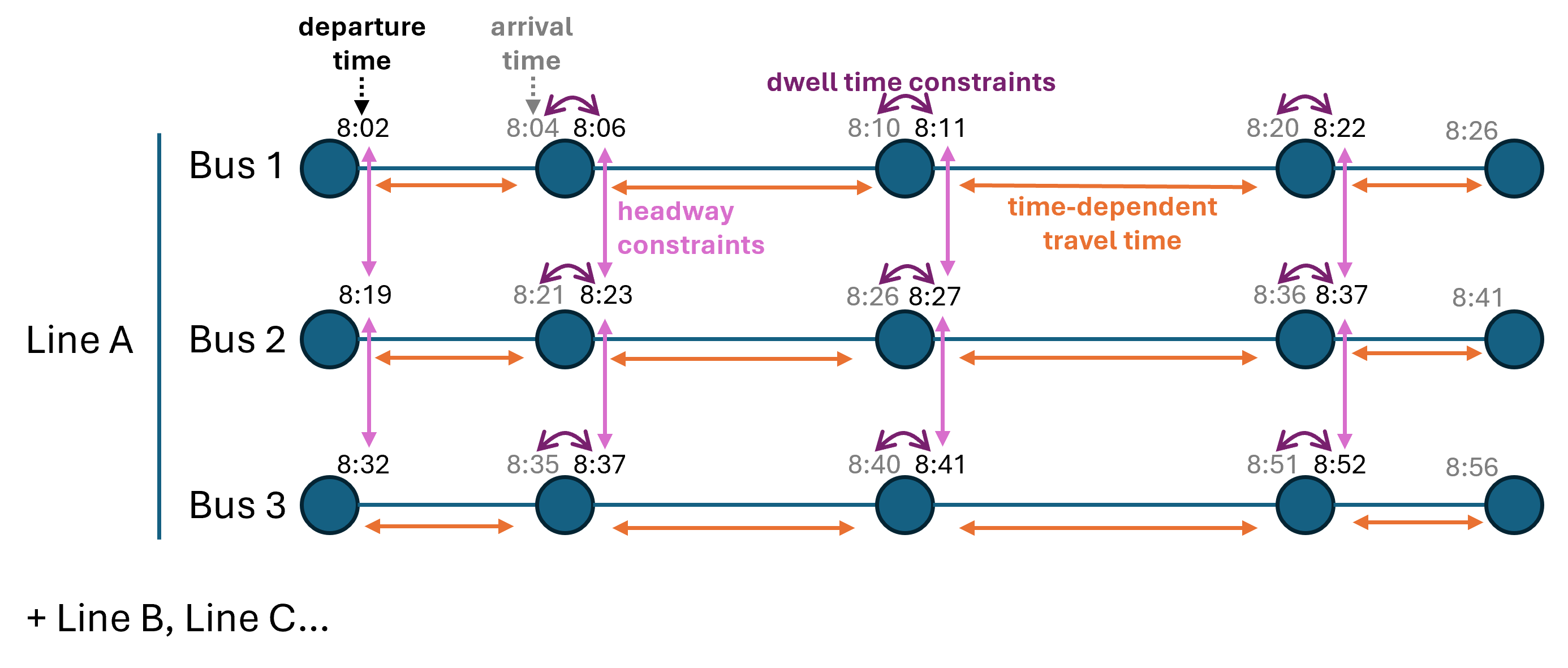
Decision Variables (Mixed Lines)
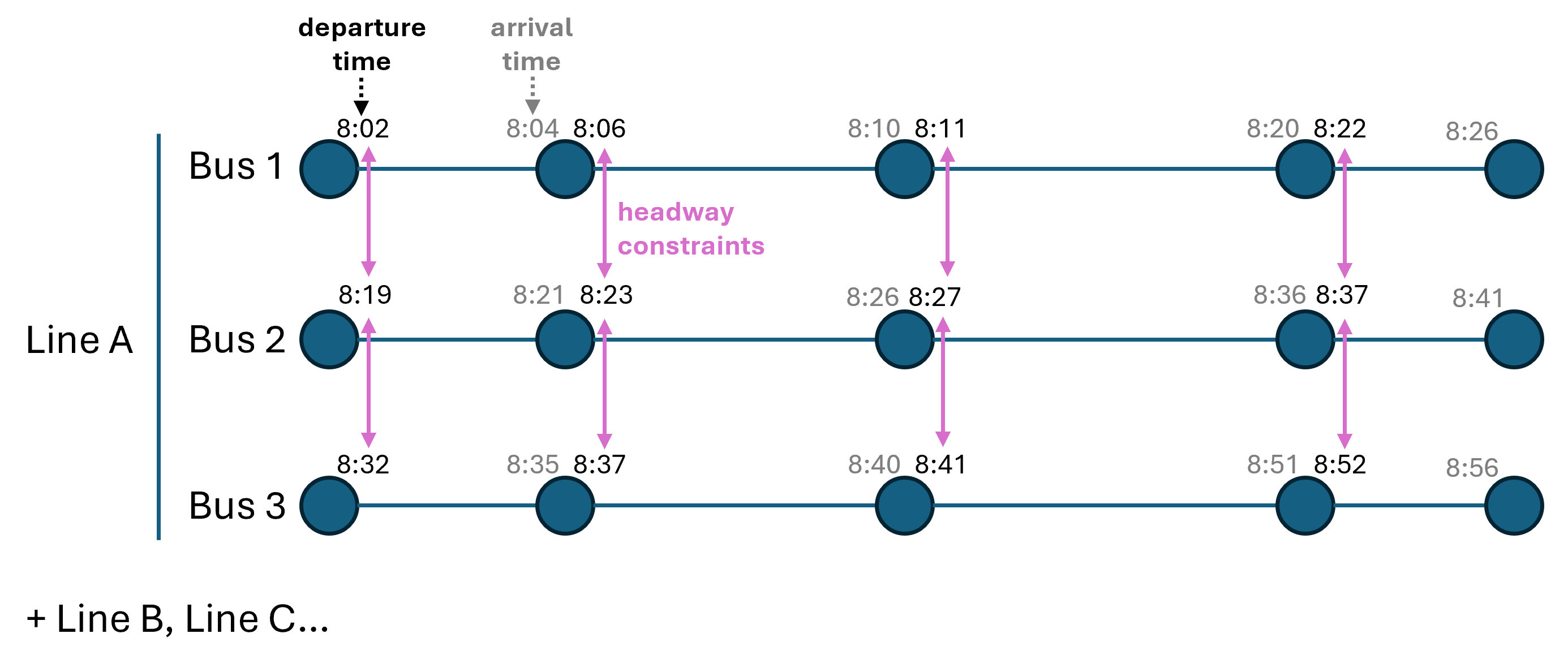
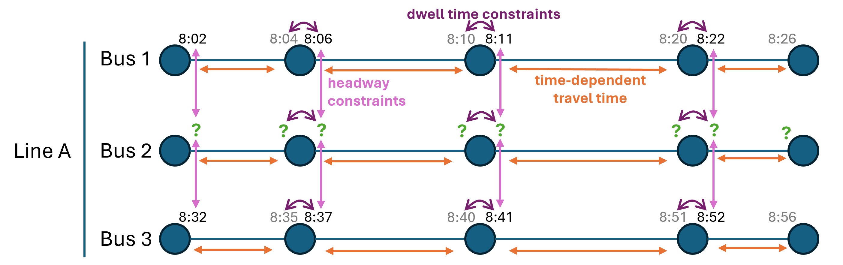
Constraints: Headway
Constraints: Dwell Time
Constraints: Comprehensive
Model Summary
Key components of the timetabling model
- Decision variables: Departure times from each stop for each bus
- Constraints:
- Min/Max headways between consecutive buses
- Min/Max dwell times at stops
- Travel time consistency
- Objective: Minimize weighted passenger travel times
Large Neighbourhood Search Principles
- Metaheuristic: Iterative improvements until limit reached
- Destroy then Repair: At each iteration, part of the solution is destroyed then reconstructed
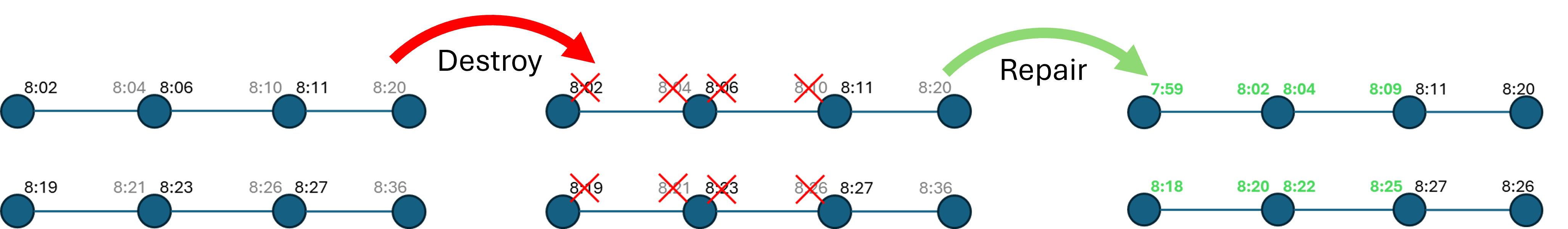
Destroying vs Repairing
Destroying is easy...
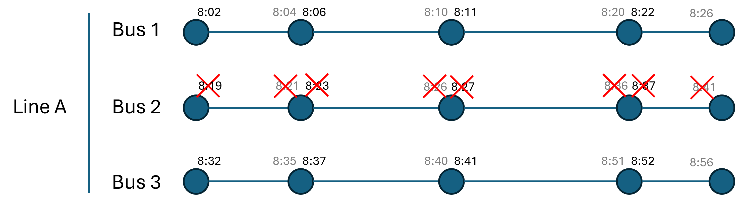
...repairing is difficult!
- Hard to guide heuristic repairs
- Often produce unfeasible timetables
MILP Repair Operator
- Solve a restricted problem with a Mixed-Integer Linear Programming (MILP) solver
- Acts like solving the model with a restricted set of decision variables
MILP vs Heuristic Repair
| Feature | MILP Repair | Heuristic Repair |
|---|---|---|
| Produce feasible solutions | Always | Sometimes |
| Produce improving solutions | Sometimes | Very rarely |
| Speed | Slow | Fast (20,000×) |
| Most efficient... | End of run | Beginning of run |
Key Insight: Use Adaptive Large Neighbourhood Search to leverage both!
Standard ALNS Probabilities
- Scores: $s_1, s_2, \dots$ indicate quality of solutions
- Weights: Selection probability is proportional to score
Standard Formula
\[ p_i = \frac{s_i}{\sum_k s_k} \]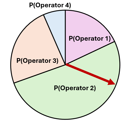
Intuitive Idea: Why $s_i/t_i$ Fails
Assume two operators $i$ and $j$:
- $s_i = s_j$
- $t_i = 1$ ms, $t_j = 99$ ms
- $i$ is 99× more efficient than $j$
Result
- $i$ used 99% of iterations
- But $j$ takes 99× more time per iteration
- 50% of time is wasted on operator $j$!
The Inverse-Square Rule
- Time distributed proportionally to $s/t$
- This requires weights to be $s / t^2$
Inverse-Square Rule
\[ p_i = \frac{s_i / t_i^2}{\sum_k s_k / t_k^2} \]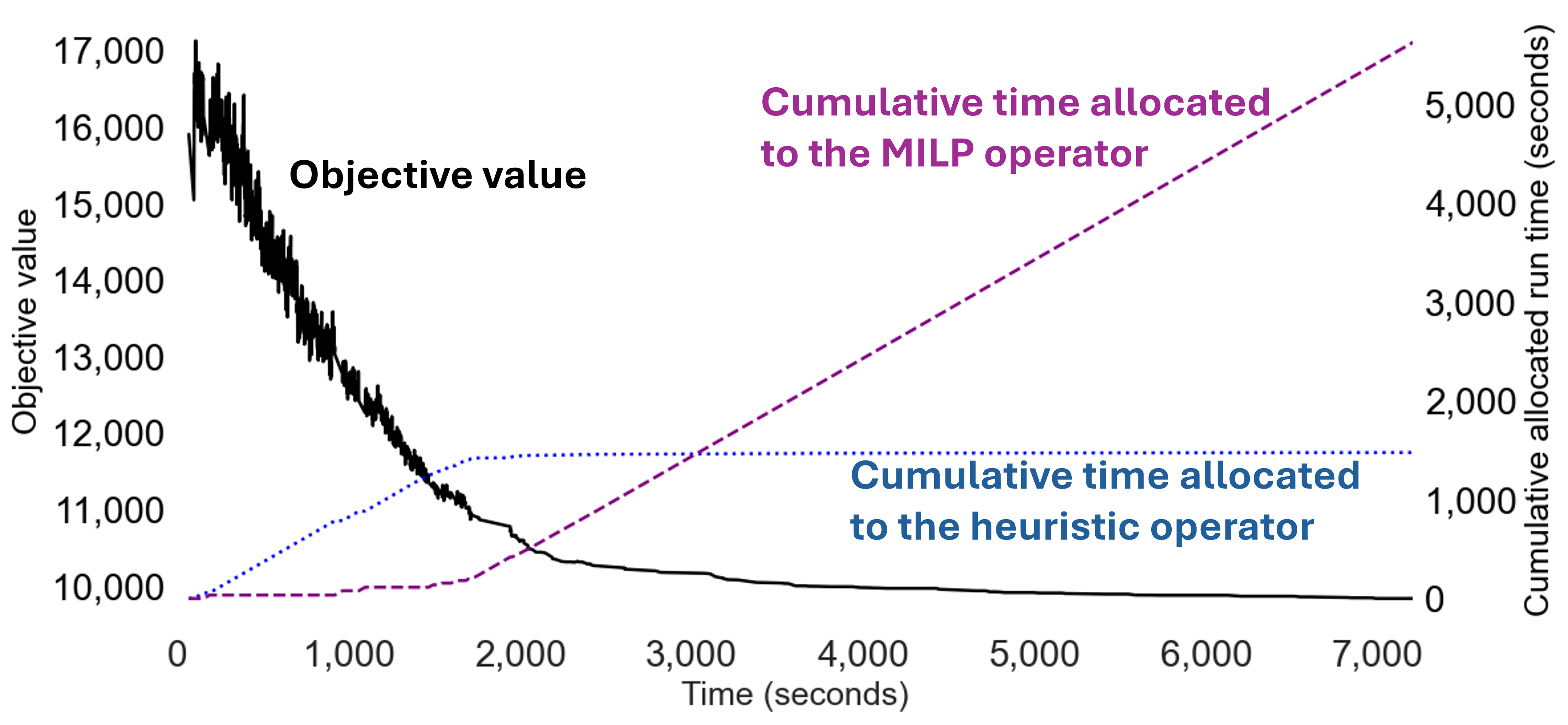
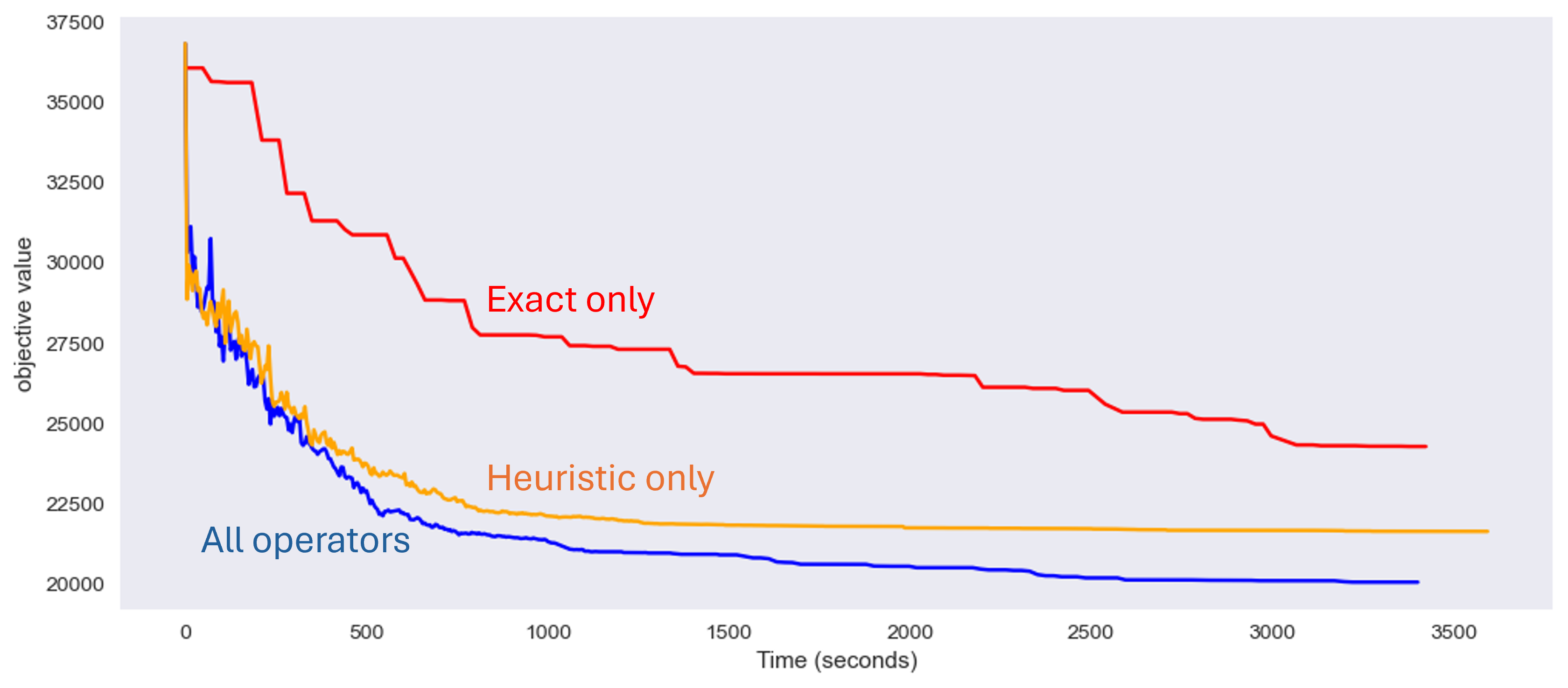
Typical Runs Comparison
Inverse-Square Rule Results
| Size | vs Standard ($s_i$) | vs Linear ($s_i/t_i$) | vs Cubic ($s_i/t_i^3$) |
|---|---|---|---|
| Small | 0.3% - 0.6% | 0.0% - 0.4% | 4.6% - 6.5% |
| Medium | 0.6% - 0.8% | 0.4% - 0.7% | 6.1% - 6.2% |
| Large | 0.7% - 1.8% | 1.2% - 2.0% | 2.2% - 3.1% |
Synergy: MILP + Heuristic
| Size | Both vs Heuristic only | Both vs MILP only |
|---|---|---|
| Small | 4.5% - 6.6% | 0.2% - 0.7% |
| Medium | 7.0% - 8.1% | 0.6% - 1.0% |
| Large | 2.9% - 4.1% | 1.6% - 2.0% |
Conclusion
- Identified Issue: Standard ALNS has issues with mixed operator speeds.
- Inverse-Square Rule: $p_i \propto s_i / t_i^2$ correctly allocates time.
- Synergy: MILP + Heuristic operators are highly complementary.

Thank you!
Questions?
www.dryujiang.uk